Conditional Generation of Medical Images using VAE
Overview
Conditional generation of medical images across different modalities and classes is crucial for data augmentation, training robust medical AI systems, and understanding cross-modal relationships in medical imaging. We address this challenge using a conditional Variational Autoencoder (CVAE) that integrates both class and modality conditioning through embedding layers. Our architecture includes auxiliary classifiers to structure the latent space, enabling controlled generation across three medical imaging domains: PathMNIST (tissue pathology), TissueMNIST (kidney cortex), and OCTMNIST (retinal OCT). The model successfully generates distinguishable samples across different modalities with excellent reconstruction quality and clear modality separation in latent space. However, class-conditional generation remains challenging due to poor class separation and auxiliary classification performance across 352K samples spanning 21 diagnostic classes. This work was completed as a course project for "Deep Generative Models".
Method
Dataset
Training is performed on 352,939 total samples with the following per-dataset breakdown: PathMNIST (89,996 training, 7,180 test), TissueMNIST (165,466 training, 47,280 test), and OCTMNIST (97,477 training, 1,000 test samples). The datasets are mapped to 21 global classes with PathMNIST classes 0-8, TissueMNIST classes 9-16, and OCTMNIST classes 17-20.
Conditional VAE Architecture
Starting from a single-channel $28\times 28$ pixel image, three convolution layers are applied, going from $1\to32\to64\to128$ channels while reducing image size from $28\to14\to7\to3$. We use a kernel size of 4, a stride of 2 and a padding of 1. Every convolutional layer is followed by batch normalization and leaky ReLU.
The conditional information is integrated through embedding layers: class labels are mapped to 128-dimensional embeddings and modality labels to 64-dimensional embeddings. The output of the last convolutional layer is flattened (yielding 1152 features) and concatenated with the 192-dimensional conditional embedding vector, resulting in a 1344-dimensional combined representation. This is passed through a 256-dimensional linear layer and then through two linear layers for $\boldsymbol\mu$ and $\log\boldsymbol\sigma$ to map to the 128-dimensional latent distribution.
The decoder mirrors this process: latent codes are concatenated with the same conditional embeddings before being passed through the decoder network. Additionally, we include auxiliary classification heads that predict class (21-way classifier) and modality (3-way classifier) from the latent mean $\boldsymbol\mu$. The class predictor uses layers of dimensions $64 \to 128 \to 64 \to 21$ with batch normalization, leaky ReLU, and dropout (0.3, 0.2). The modality predictor uses $64 \to 64 \to 3$ with similar regularization.
The final conditional VAE model has a total of 1,155,993 parameters.
Conditional VAE Loss Formulation
The loss is composed of several components:
- MSE Loss ($\mathcal{L}_\text{MSE}$): Measures reconstruction on raw pixels
- L1 Loss ($\mathcal{L}_\text{L1}$): Alternative reconstruction loss that promotes sharper reconstructions and is more robust to outliers than MSE
- Perceptual Loss ($\mathcal{L}_\text{Perceptual}$): Like MSE but instead of using raw pixels, it uses feature maps extracted by a separate untrained and frozen Convolutional NN (architecture: Conv2d(1→16, k=3) → ReLU → Conv2d(16→32, k=3) → ReLU → AdaptiveAvgPool2d(7)), applied to both ground truth and generated image
- KL Loss ($\mathcal{L}_\text{KL}$): Standard VAE KL divergence loss ensuring latent distributions match the prior
- Class Classification Loss ($\mathcal{L}_\text{Class}$): Cross-entropy loss for predicting the correct class label from the latent representation
- Modality Classification Loss ($\mathcal{L}_\text{Modality}$): Cross-entropy loss for predicting the correct imaging modality from the latent representation
The total loss is composed as:
\(\mathcal{L}_\text{total} = \mathcal{L}_\text{VAE} + \mathcal{L}_\text{aux}\)
where:
\[\begin{align} \mathcal{L}_\text{VAE} &= \underbrace{\alpha_\text{MSE}\cdot\mathcal{L}_\text{MSE} + \alpha_\text{L1}\cdot\mathcal{L}_\text{L1} + \alpha_\text{Perceptual}\cdot\mathcal{L}_\text{Perceptual}}_{\text{Reconstruction Loss}} + \beta\cdot\mathcal{L}_\text{KL}\\ \mathcal{L}_\text{aux} &= \gamma \cdot (\mathcal{L}_\text{Class} + \mathcal{L}_\text{Modality}) \end{align}\]Hyperparameters
The loss weights and training schedule are as follows:
- $\alpha_\text{MSE} = \alpha_\text{L1} = 0.4$: Equal weighting for pixel-level reconstruction losses
- $\alpha_\text{Perceptual} = 0.1$: Lower weight for perceptual loss to complement pixel losses
- $\beta$: KL loss weight with linear warm-up schedule from 0 to $\beta_\text{max} = 0.001$ over 20 epochs
- $\gamma = 1.0$: Weight for auxiliary classification tasks
Training Schedule
The KL term $\beta$ follows a linear warm-up schedule:
\[\beta(t) = \begin{cases} 0 & \text{if } t < t_\text{warmup} \\ \beta_\text{max} \cdot \frac{t - t_\text{warmup}}{t_\text{schedule}} & \text{if } t_\text{warmup} \leq t < t_\text{warmup} + t_\text{schedule} \\ \beta_\text{max} & \text{if } t \geq t_\text{warmup} + t_\text{schedule} \end{cases}\]with $t_\text{warmup} = 20$ epochs and $t_\text{schedule} = 100$ epochs.
Training Details
We train using the Adam optimizer with learning rate of $5 \times 10^{-4}$ and weight decay $1 \times 10^{-5}$ for 150 epochs with batch size 256. The learning rate follows a ReduceLROnPlateau schedule (patience=8, factor=0.5) and gradients are clipped to maximum norm 1.0. The model uses latent dimension $d_z = 128$ with class embeddings $d_c = 128$ and modality embeddings $d_m = 64$.
Results
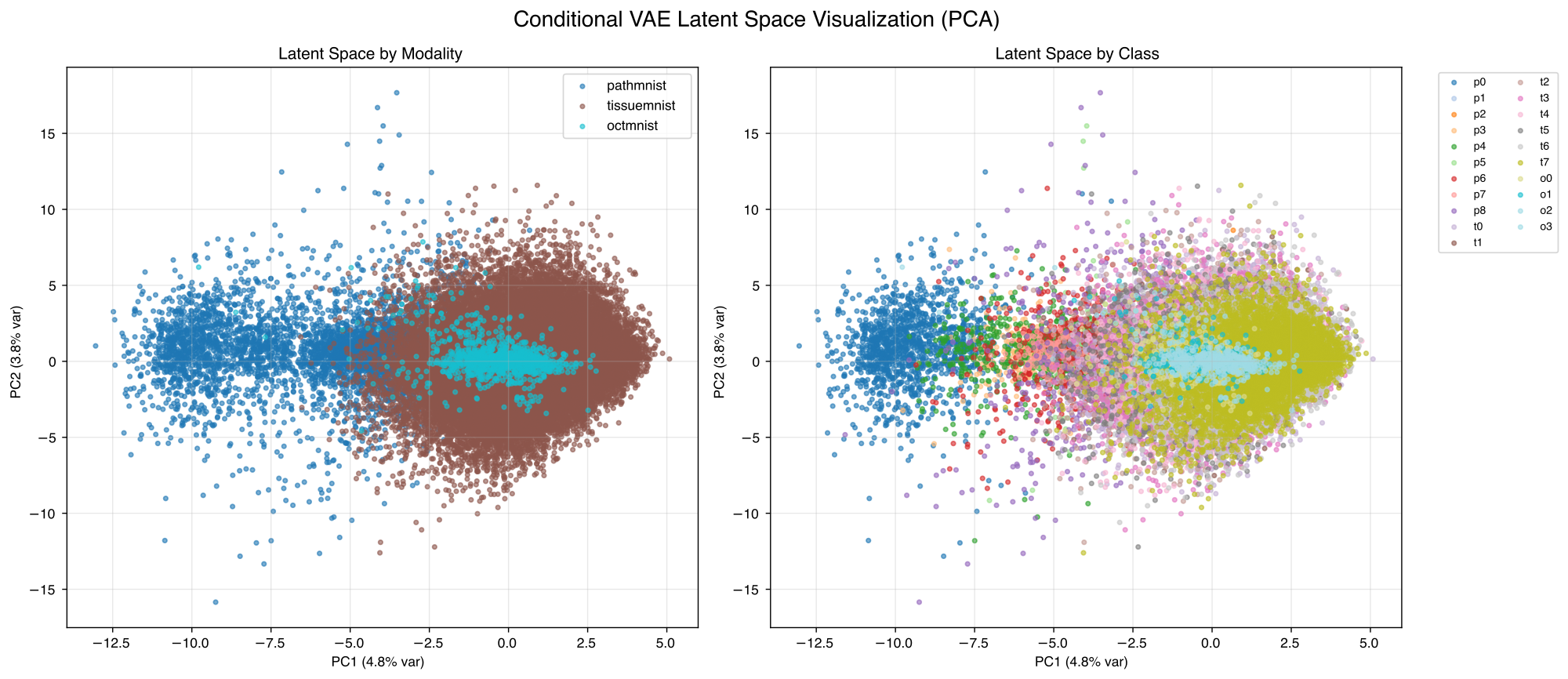
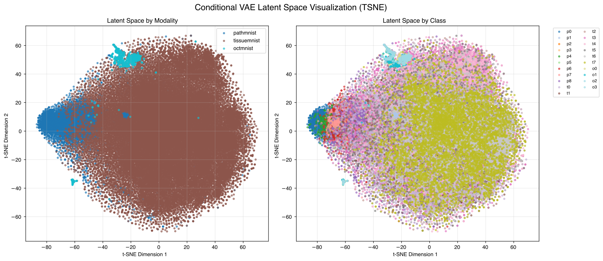
In figure 1 we can see that the model converges quite fast and with best model selection we get the best results after 79 epochs, which we also show the later results for. Figure 2 shows some reconstruction examples from the PathMNIST subset that work quite well. Figure 3 depicts generated samples for the different modalities and different classes within the modalities. We can observe that the different modalities are distinguishable, see figure 6 for comparison to real samples. We can see that the overall appearance of the generated samples reflects the real sample structure. Figures 4 and 5 show visualizations of the latent space after training. We can see that the modalities are separated quite well while the classes are highly overlapping.
Some important findings are that the loss reduces significantly when using a latent dimension of 128 instead of 64, while scaling up the model with more convolutional layers (roughly 4.8 million parameters) leads to results looking very similar to what we already had, so we assume our network already has good capacity.
One significant limitation we still have is that our auxiliary tasks perform very poorly. Class classification accuracy gets stuck around 34% and modality classification gets stuck at around 39% (almost random probability), despite clear visual modality clustering in latent space. It is not clear where this issue arises from but it might be related to the balancing of different loss components.